Welcome to part 6 in my classification blog series! In part 1, we loaded a decade’s worth of group chat messages into Python, in part 2 we learned how to quantify model accuracy and tested that knowledge with a basic model, in part 3 we dug into our data to extract the features we’ll need for our models, in part 4 we built a linear model and compared that to the naive model from part 2, and in part 5 we did an overview of basic neural networks and implemented one to mimic our linear model.
In this post, we’ll go one step further and implement a neural net with more than one layer (called a multi layer perceptron or MLP) to classify our messages.
Disclaimer that gets more relevant with each post: I’m not a math major nor someone deeply steeped in the theory, so I’ve been and will continue to keep my explanations in this series high level. If you want to learn more about anything in this series, YouTube and ChatGPT are your friends. There are likely many things I’m wrong about in this series, so if you see something that is off base or flat out incorrect please let me know and I’ll do my best to fix it.
Beyond linear models
In the last two posts, we built models that were linear in nature. That means that the model’s output was a linear combination of the inputs. This works well in certain cases (indeed, in our case it works better than you might expect), but is overall a very limiting way to think about our data. Check out section 5.1.1.1 from this textbook for a more in depth look at how linear models fall short.
If you are thinking about our structure from last time, you may suggest that we simply add another layer of neurons and connections in between in the input and output. This is closer to what we want, but we still have a problem. If we add a layer of neurons and connections, we still have a linear model. The output of the first layer is a linear combination of the inputs, and the output of the second layer is a linear combination of the first layer’s outputs. If you carry out the math you can show that a single linear layer and multiple linear layers are functionally identical in terms of the types of relationships that they can model.
To create a neural net that is more powerful than a linear model, we need some way to introduce non-linearity into our model. A common way to solve this is to pass each neuron to an “activation function” after each linear layer to increase the predictive capability of the model. Essentially, this takes the output of each neuron and passes it to a function (common choices include ReLU, Sigmoid, and Tanh) so that the result is non-linear. We’ll try a few different activation functions in the code below to see how they compare performance wise. Check out sections 5.1.1.3 and 5.1.2 for a deeper explanation of activation functions.
Now, our multi-layered neural net (called a multilayer perceptron) looks like this:
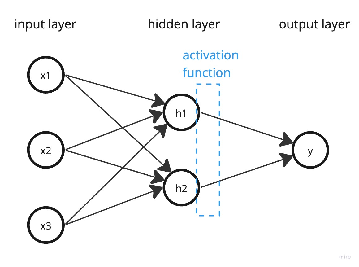
You can have as many hidden layers, inputs, and outputs as you want. In practice (according to my reading), deeper networks (more layers) are more powerful than wider networks (more nodes per layer), but there are tradeoffs and that’s just a rule of thumb.
Training gets more computationally intense as a result of the activation function (activation layers add depth to the network, increasing the number of steps in backpropagation) and multiple layers (now we need the chain rule of calculus to calculate gradients), but I won’t get into the math here since the packages do it automatically for us. Check out section 5.3 if you want to learn more about the math.
As we increase the complexity of our models, we’ll also start to see a greater incidence of overfitting our training data. If we encounter overfitting with this model, I’ll briefly explain any “regularization” steps we take to combat it. Regularization techniques, like dropout or L2 regularization, can help prevent the model from fitting the noise in the training data and improve generalization to unseen data.
MLP implementation
Thanks to PyTorch and similar packages, implementing the MLP is straightforward. We’ll start with two hidden layers and the ReLU non-linear activation function. We’ll also stick with the Cross Entropy loss function and the Adam optimizer from the linear NN code. Here’s our initialization code:
 1def __init__(self, input_features, num_classes, hidden_neurons=32):
 2    # Define the network layers
 3    self.net = nn.Sequential(
 4        nn.Linear(input_features, hidden_neurons),
 5        nn.ReLU(),
 6        nn.Linear(hidden_neurons, hidden_neurons),
 7        nn.ReLU(),
 8        nn.Linear(hidden_neurons, num_classes)
 9    )
10
11    # Define the loss and the optimizer
12    self.criterion = nn.CrossEntropyLoss()
13    self.optimizer = optim.Adam(self.net.parameters())
We’ll likely add some more code to this initialization to correct for overfit, which I’ll explain as we test and train this model. The creation code is remarkably similar to the linear NN code, just with different layers in the nn.Sequential() call.
Since our neural net has the same number of inputs and outputs as the linear NN, we can use nearly identical training and prediction code. Here’s the basic training code:
 1def train_model(self, train_data, train_labels, epochs=100):
 2    self.trained = False
 3    train_data = torch.FloatTensor(train_data)
 4    train_labels_indices = torch.argmax(train_labels, dim=1)
 5    train_labels = torch.LongTensor(train_labels_indices)
 6
 7    for epoch in range(epochs):
 8        self.optimizer.zero_grad()
 9        output = self.net(train_data)
10        loss = self.criterion(output, train_labels)
11        loss.backward()
12        self.optimizer.step()
13
14        if epoch % 10 == 0:
15            print(f'Epoch {epoch+1}/{epochs}, Loss: {loss.item()}')
16
17    self.trained = True
Similarly to the initialization, this code will get more complicated as we add regularization (overfitting protection), but for now it’s pretty simple. We convert our data to PyTorch tensors, then loop through our training data. For each epoch, we zero out the gradients (in essence make the gradients forget the last round of training), calculate the output of the network, calculate the loss, calculate the gradients, and then update the weights. We also print out the loss every 10 epochs so we can see how the model is improving over time.
Here’s the prediction code:
 1def predict(self, data):
 2    if not self.trained:
 3        raise RuntimeError("Model must be trained before prediction.")
 4
 5    with torch.no_grad():
 6        data = torch.FloatTensor(data)
 7        output = self.net(data)
 8        probabilities = nn.functional.softmax(output, dim=1)  # Convert output to probabilities
 9
10    return probabilities
This code is identical to the linear NN code. You can find the full code (updated with any additional techniques) on Github.
Testing the MLP
The code above will run and can be used with our existing feature extraction and ClassifierEvaluator code. But it falls short on performance because it overfits the training data when trained for long enough to be accurate. Here are the various techniques I used to improve the performance of the MLP:
- Normalize the features - I used the same normalization from the linear NN and linear model code. Having all the features on the same scale helps the model converge faster and helps the gradients be of the same magnitude which makes training more “fair” to each weight.
- Trained on minibatches - Instead of training on the entire dataset at once, I trained on smaller portions of the data at a time. Minibatch training is typically more effective at combatting overfit than full batch training, converges faster than training on one data point at a time, and is more computationally efficient for calculating gradients than full batch training.
- Added weight decay - This adds a term to the loss function that penalizes extreme weights to help prevent overfitting. We use l2 regularization for no particular reason other than that it is standard.
- Added batch norm layers - Prevent the distribution of the weights from shifting too much during training. This means that deeper layers don’t have to “relearn” the distribution of the previous layers’ weights as often so can converge faster. This is explained fully in Andrej Karpathy’s Neural Networks: Zero to Hero series.
- Added dropout - This randomly chooses a certain percentage of the neurons in each layer to be ignored (zeroed or dropped out) during each batch of training. This helps prevent overfitting by ensuring that the model doesn’t rely too heavily on any single neuron.
In a nutshell, I approached training the neural net by hyperparameter tuning (changing learning rate, number of nodes, etc.) until it overfit the training data or performance plateaued, then I’d add or tune a regularization technique to reduce overfit without harming performance. To illustrate the benefit of testing on your dataset instead of blindly following best practice, when I added batchnorm into the model, it actually increased rather than decreased overfit without a noticable difference in test accuracy performance.
I experimented pseudo-scientifically with each of my hyperparameters and regularization techniques to find the best model (you can see my ugly test code here). With each subset of combinations, I seemed to reach a local maximum of performance right around 51% testing accuracy (training accuracy sometimes was much higher). The fact that I hit this with multiple combinations makes me think that I’ve hit the upper limit given the specific features I’ve extracted so far.
The final model I landed on had the following characteristics:
- no dropout or batchnorm
- 64 hidden neurons per hidden layer (128 total)
- 1e-4 weight decay (L2 regularization)
- 0.99 momentum with step size 100 (i.e. multiply the learning rate by 0.99 every 100 minibatches)
- 100 epochs with minibatch size 128
- ReLU activation function
The resulting model had a final testing accuracy of just over 51%. (Compare to 45% accuracy with the linear model and 42% accuracy with the linear NN.)
You can find the full model code here and testing code here.
Conclusion
In this post, we built a multi layer perceptron to classify our messages. We learned about the limitations of linear models and how to add non-linearity to our models to improve performance. We also learned about some of the techniques we can use to combat overfitting and how to tune our models to get the best performance.
We maxed out our performance on these features at just over 51% testing accuracy. In the next post, we’ll either add more features, dive into analyzing the network, or try a more advanced model architecture depending on what I learn next.