Welcome to part 5 in my classification blog series! In part 1, we loaded a decade’s worth of group chat messages into Python, in part 2 we learned how to quantify model accuracy and tested that knowledge with a basic model, in part 3 we dug into our data to extract the features we’ll need for our models, and in part 4 we built a linear model and compared that to the naive model from part 2.
Today, we’re (finally) going to start deep learning! We’ll start with an overview of neural network structure, training, and application, and then we’ll build a neural network to represent our linear model from part 4.
Disclaimer that gets more relevant with each post: I’m not a math major nor someone deeply steeped in the theory, so I’ve been and will continue to keep my explanations in this series high level. If you want to learn more about anything in this series, YouTube and ChatGPT are your friends. There are likely many things I’m wrong about in this series, so if you see something that is off base or flat out incorrect please let me know and I’ll do my best to fix it.
What is a neural network?
At this point, I highly recommend stopping my blog series and watching at least the first video from Andrej Karpathy’s Neural Networks: Zero to Hero series It’s a great overview of what neural networks are and how they work. You can also follow along with my code from the lectures, which I tried to comment up a bit more than Andrej’s code from the series. If you want a little less intense of an introduction, this video is a good overview of the basics, but I found it easier to understand after Andrej’s deep dive.
You can think of a neural network as a way to represent a giant system of equations that estimates some (usually) real world function. It is comprised of nodes (also called neurons) connected to other nodes with edges. Nodes are typically arranged in groups or “layers” that are connected to each other with edges, each of which has a weight associated with it. The first layer of a neural network represents the inputs to the neural net and the last layer represents the output. As an example, consider the following neural network that represents the price of a house (the output) as a function of the number of bedrooms and square footage (the inputs):
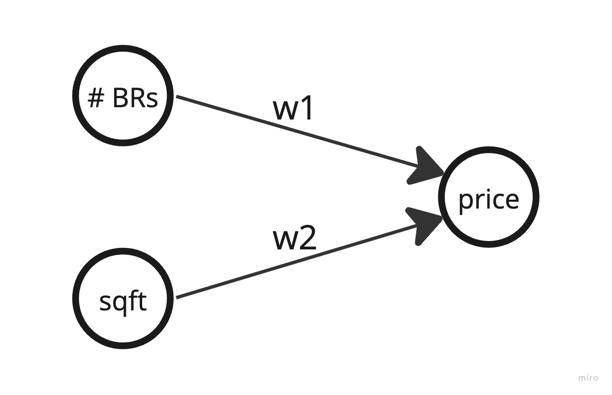
This neural net represents the equation #bedrooms * w1 + sqft * w2 = price. The goal of the neural net is to estimate the relationship between the number of bedrooms, square footage, and price by learning the value of the weights. So, how does it learn?
Training a neural network
The neural net learns by passing data through it and adjusting the weights based on the error between the output of the neural net and the actual value. For example, if we pass in a house with 3 bedrooms, 2000 square feet, and a price of $500k, the neural net will calculate 3 * w1 + 2000 * w2 = price. If the price it calculates is $400k, it will adjust the weights to increase the price it calculates. If the price it calculates is $600k, it will adjust the weights to decrease the price it calculates.
To know how much to adjust the weights by, we use a “loss function” to calculate the error between the output of the neural net and the actual value. The loss function is a function of the weights and the inputs that are passed into the neural net. We can estimate how much each weight impacts the loss function by changing the weight by a small amount and seeing how the loss function changes, similar to estimating a derivative numerically in calculus. In the example above, let’s assume we had the price per bedroom w1 of $50k and the price per square foot w2 of $200. For our 3br 2000sqft house, that would lead to a price of 3 * $50k + 2000 * $200 = $550k. For a simple example, we’ll set the loss function to be the sum of squared errors, so our loss would be (550k - 500k)^2. If we slightly increase either the price per square foot or the price per bedroom, the predicted price would go up and our loss function would increase. This tells us that we can reduce the loss function by decreasing the value of the weights in our equation, and the amount we decide to change each one is proportional to how much each weight impacts the loss. For example, if we changed the $50k price per bedroom and $200 price per square foot by $1 each, the change to the price per square foot would have a much larger impact on the final price ($2000 vs $3) and thus a much large impact on the loss function.
Usually, you’d want to adjust the weights based on a number of input examples instead of just one, and running all those calculations to estimate how much to change each weight can get expensive. Instead of numerically estimating, then, we can also design the loss function and layers such that we can calculate the gradient, or partial derivative with respect to each weight, of the loss function. We then slightly decrease each weight by the corresponding gradient to lower the loss function. This is called gradient descent and the magnitude of the change you make to each variable is called the learning rate. There’s some really cool math that happens here, so I recommend watching the videos above.
By running this process of gradient descent over and over again on our training data, updating the weights each iteration, we can estimate the weights that minimize the loss function.
Watch Andrej Karpathy’s Neural Networks: Zero to Hero series for a better explanation of neural nets and gradient descent (and everything else in this post).
Neural nets for classification
The above explanation makes sense for numeric estimation problems with only one output, but what about the classification problems we’re dealing with? We treat these problems very similarly to how we treated the linear representation of classification problems: output a probability for each class from the neural net and then choose the class with the highest probability. The major change we need to make here is converting the output for each class, which is a regular number, into a probability between 0 and 1. It is standard to use the softmax function for this. Softmax normalizes a set of values to be between 0 and 1 using the exponential function. Check out the link or ask ChatGPT if you want to learn more.
This explanation was a very basic intro to neural nets, but there is lots more that I didn’t cover (like activation functions). We may cover that as it comes up in future models, or we may ignore it altogether. Check out the resources above if you want to learn more.
Implementing a simple linear classifier as a neural net
From the explanation above, you saw that we can make represent a system of equations (like our linear model from part 4) as a neural net. The input layer of nodes will have one node for each feature and the output layer will have one node for each class that we are predicting. Each node in the input layer will be connected to each node in the next layer.
Note: as part of parameter tuning to get these models to perform as well as our linear models, I had to use a number of techniques that I didn’t cover above like minibatches and learning rate decay. If you watched the videos above you know what those are, but if not the full code might not make sense. I tried to comment the code as best I could to explain these techniques. I simplified the code below to be easy to understand and not include all of that complexity. I think the code below should still work if you run it, it’ll just perform poorly.
To create our neural net model:
1def __init__(self, input_dim, output_dim):
2    super().__init__()
3    self.model_type = "MultiClassLogisticNN"
4    self.net = nn.Linear(input_dim, output_dim)  # Only input and output layers
5    self.criterion = nn.CrossEntropyLoss()
6    self.optimizer = optim.Adam(self.net.parameters())
The neural net itself is only a single linear layer. We also choose the loss function we will use (self.criterion) and set the optimizer that will decide how to adjust the parameters based on the loss function (self.optimizer).
To train the neural net:
 1def train_model(self, train_data, train_labels, epochs=2000):
 2    self.trained = False
 3    train_data = torch.FloatTensor(train_data)
 4
 5    train_labels_indices = torch.argmax(train_labels, dim=1)
 6    train_labels = torch.LongTensor(train_labels_indices)
 7
 8    for epoch in range(epochs):
 9        self.optimizer.zero_grad()
10        output = self.net(train_data)
11        loss = self.criterion(output, train_labels)
12        loss.backward()
13        self.optimizer.step()
14        print(f'Epoch {epoch+1}/{epochs}, Loss: {loss.item()}')
15
16    self.trained = True
We transform the input data and labels into the right format and datatype. Do a “forward pass” over the net to generate the output (i.e. put the inputs in the neural net and do the calculations to get the output), calculate the loss using our criterion, do a “backwards pass” or back propagate to calculate the gradient for each of the weights, “step” the optimizer to actually update the weights, and then repeats that epoch number of times.
To predict the neural net:
 1def predict(self, data):
 2    if not self.trained:
 3        raise RuntimeError("Model must be trained before prediction.")
 4
 5    with torch.no_grad():
 6        data = torch.FloatTensor(data)
 7        output = self.net(data)
 8        probabilities = F.softmax(output, dim=1)  # Apply softmax to convert output to probabilities
 9
10    return probabilities
Prediction is simply does a forward pass through the net and converts the results into probabilities using the softmax function explained above. Note that it sets torch.no_grad() to prevent the neural net from calculating the gradients used to train the model. This is mostly for computational efficiency.
You can see the full code with all the tweaks not mentioned here on Github.
Using the linear classifier neural net
Neural Nets are finnicky and take some tuning to optimize the “hyperparameters” like the number of layers, nodes per layer, learning rate, etc. It took me some time to get this simple net to match the performance of our linear models. I had to add parameter normalization, increase the number of epochs, add interaction features (typically that is handled implicitly by the layers of the network but can’t be in this simple one layer model), add mini-batches for training, and change the learning rate decay. After some trial and error, I managed to build a model that mostly matched the performance of our previous models:
| Model Description | Training Accuracy (Linear) | Training Accuracy (NN) | Testing Accuracy (Linear) | Testing Accuracy (NN) |
|---|---|---|---|---|
| Only the two most important features | 0.4127 | 0.4146 | 0.4036 | 0.4032 |
| Any feature with comparatively high effect size | 0.4255 | 0.4296 | 0.4106 | 0.4144 |
| All features | 0.4376 | 0.4371 | 0.4264 | 0.4257 |
| Only the two most important features and their interactions | 0.4177 | 0.4220 | 0.4087 | 0.4129 |
| Any feature with comparatively high effect size and their interactions | 0.4714 | 0.4438 | 0.4510 | 0.4279 |
For all but the final, most complex model (recall this had 552 features) the performance is comperable between the two types of models! This implies that our neural nets are doing a good job of approximating the weights for the linear equations. We could try to tune the parameters a bit more to get the final model to match, but that’s not the point of the series so I’ll leave it here for now.
You can see the full testing code here on Github.
Conclusion
We’ve finally started deep learning!
To recap, we explained the basic structure of a neural net and its components. We built a neural net for our linear model and learned how to train and use that neural net. We saw that the neural net was able to approximate the linear model weights pretty well once we tweaked the hyperparameters like learning rate.
In the next post, we’ll start to build more complex neural nets.