Welcome to part 4 in my classification blog series! In part 1, we loaded a decade’s worth of group chat messages into Python, in part 2 we learned how to quantify model accuracy and tested that knowledge with a basic model, and in part 3 we dug into our data to extract the features we’ll need for our models.
Today, we’re going to build a model one level up from the naive model in part 2 - a linear model.
Disclaimer that gets more relevant with each post: I’m not a math major nor someone deeply steeped in the theory, so I’ve been and will continue to keep my explanations in this series high level. If you want to learn more about anything in this series, YouTube and ChatGPT are your friends. There are likely many things I’m wrong about in this series, so if you see something that is off base or flat out incorrect please let me know and I’ll do my best to fix it.
Background and intuitive explanation
If you already understand linear models or don’t care about theory you can skip down to the next section.
Linear models are a way to represent the relationship between an input set of features and the output variable of concern. They are called “linear” models because they represent the relationship between the variables using a linear equation. Linear equations are the kind you encountered in third grade - y = m*x + b - just with more x’s. In the language we’ve been using, that translates to: y (outcome) = m (weight) * x (feature) + b (intercept/bias) where weight corresponds to the value you multiply each feature by and the intercept is the value assigned when all features = 0 (though the interpretation of what that means can get very complicated).
When our outcome variable is continuous (numerical and able to take on any value), the linear model is called a linear regression. Visualized in two dimensions (x and y, or one feature and the outcome), linear regressions look like this:
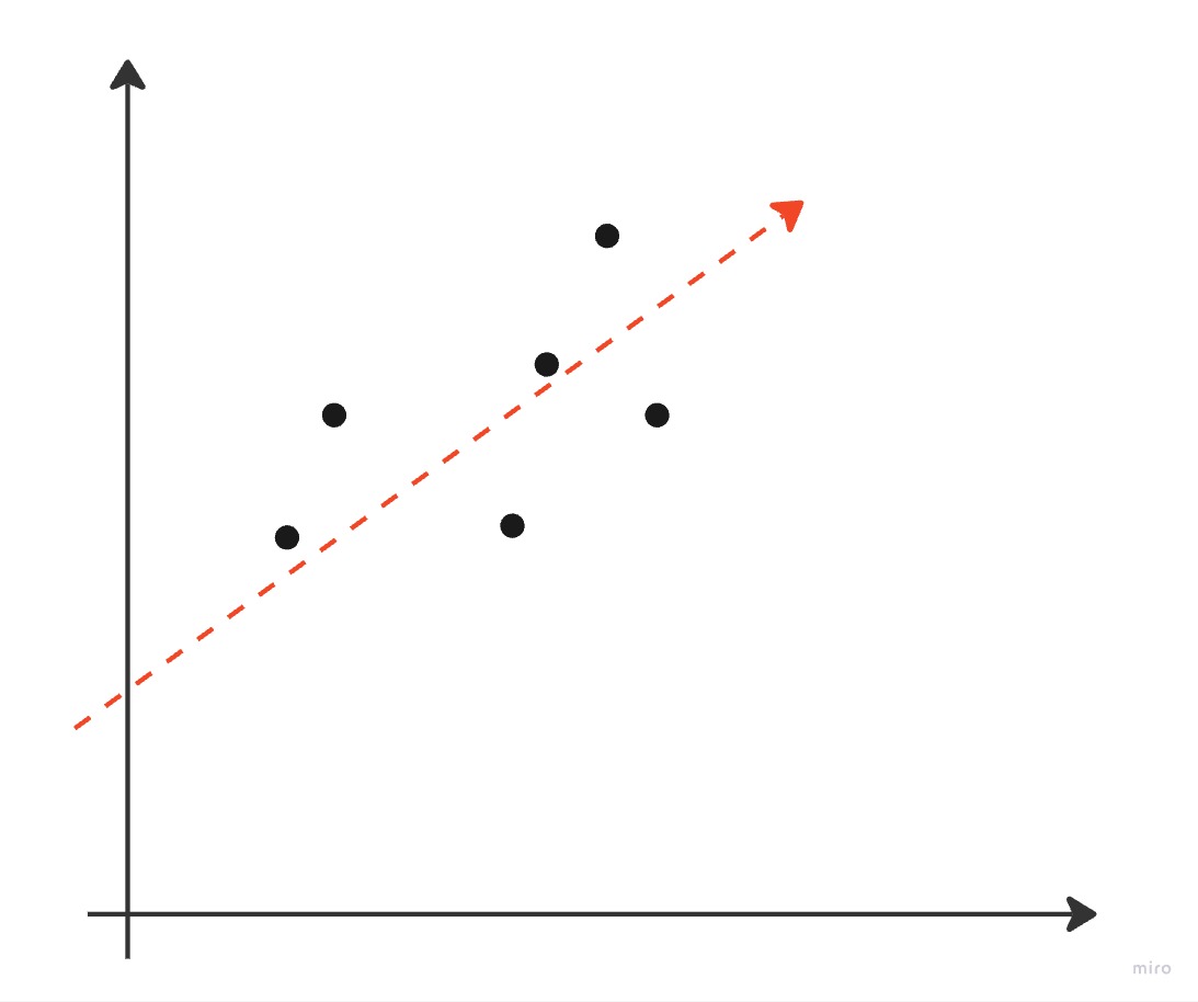
In the visualization above, the red line is the predicted values of y (aka yhat from the ClassifierEvaluator in part 2 and the points are the observed values. The model is optimized so that the difference between the red line and the points is minimized. The process is the same if there is more than one x (i.e. more than two dimensions), it is just harder to visualize: given your input of x’s (features), assign weights to each x such that you minimize the difference between the actual y and predicted yhat values. The interpretation of these models is also pretty simple: for each one unit increase or change in x, the outcome variable y will change by the weight amount. Figuring out how to set the weights is complicated, but smart math people have made smart math equations to do that. We won’t go into the math here.
When you change from a continuous outcome variable to a discrete one, though, the math and intuitive understanding gets harder. We’ll start with a binary outcome variable (one that can take on one of two values), which is called a “logistic regression model”:
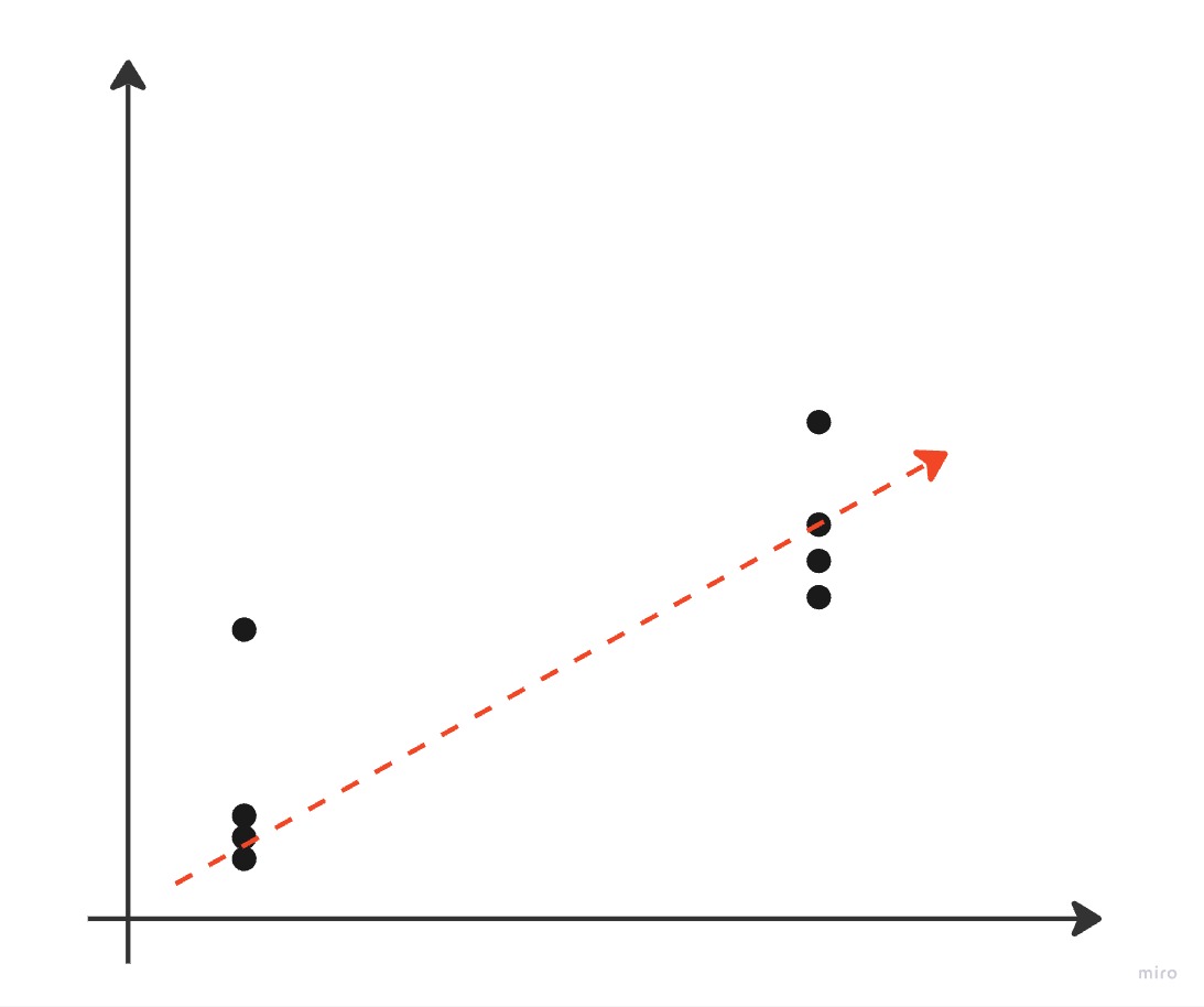
As you can see, this is a little more complicated to understand and explain. If the outcome variable can only be two values, “yes” or “no”, what does the red line mean at all points that aren’t “yes” or “no”? We explain this by using the model to calculate a probability that the outcome is “yes” or “no” rather than the value “yes” or “no” itself. We still essentially minimize the difference between the actual values “yes” or “no” and the predicted probability of “yes” or “no” occurring. We interpret the weights of this model in this way: for each one unit increase or change in x, the outcome y is weight more likely to occur. The smart math people come through again and have nice equations to calculate the weights under many circumstances.
It gets more complicated once more when we move to multiple classes:
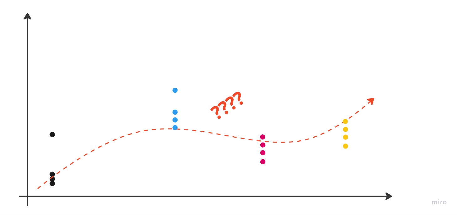
There are a number of ways to think about this problem which I won’t go into here. For our purposes, we’ll think of our multi-class linear model as producing a set of probabilities for all classes and then picking the class with the highest probability. For example, if we have three potential senders Ender, Bean, and Carn, our model would output three values: the probability that Ender, Bean, or Carn is the sender of the message. There are a variety of acceptable approaches to model this and I’ll explain the path we take in our code below.
Building a linear classifier
Hopefully the above gave you an intuitive grasp of how a linear model works. Now we turn our attention to extending the Model class from part 2 to build our own linear model for classifying messages. We’ll pick one of the many ways you can construct a linear multi-class classification model for this exercise: a one-vs-all model. In this model architecture, we compute one binary model (aka logistic regression model) for each of the classes we have, and then choose the maximum value output from those sub models as the predicted class.
Using our messages as an example, if we’re trying to predict whether Ender, Bean, or Carn sent a message we would train three binary models: one signifying “did Ender send or did someone besides Ender send it?,” another for “did Bean send or did not Bean send?,” and a third for Carn. When predicting the sender for a new message, we’d run the input through all three models and then pick the max. You can see the full code on Github; I’ll explain only the training and prediction code here. I started off building everything from scratch for you all, but after a couple of hours fighting with optimization code I caved and decided to use the scikit learn builtin logistic regression. So the extent of the math you get me to comment on for setting weights is “use a package with it builtin.”
Here is how we train each of our binary models (with some filler removed for space reasons, full code on Github):
 1from sklearn.linear_model import LogisticRegression
 2
 3def _binary_train(self, train_data, train_labels):
 4    # Train the model
 5    model = LogisticRegression(max_iter=1000, C=100.0)
 6    model.fit(train_data, train_labels)
 7    return model
 8
 9def train_model(self, train_data, train_labels, **kwargs):
10    # Compute and store the normalization parameters
11    self.feature_means = train_data.mean(axis=0)
12    self.feature_stds = train_data.std(axis=0)
13
14    # Normalize the training data
15    train_data = (train_data - self.feature_means) / self.feature_stds
16
17    for i in range(self.num_classes):
18        binary_labels = train_labels[:, i].numpy()
19        self.models[i] = self._binary_train(train_data, binary_labels)
20    self.trained = True
To train the model, we train self.num_classes (in our case 5) individual logistic regression models. This model is sensitive to the scale of variables due to some math reasons, so we also normalize the values using the standard score normalization. (To test this for yourself, clone the code and remove the normalization lines. When I did that the resulting model performed worse than the naive one.) This makes sure that all of the features we use are of roughly the same magnitude. Not pictured here, I also updated the feature extraction code so that our categorical variables like previous sender and day of week are coded in a bunch of boolean variables so that our math can handle them properly. This is similar to the one-vs-all method we are using to make the model - for the 7 days of the week, I made 7 boolean variables for isMonday, isTuesday, etc. and added them to the feature vector in place of a single day of week feature.
To predict on new data:
1def predict(self, data):
2    # Normalize data using the stored parameters
3    data = (data - self.feature_means) / self.feature_stds
4
5    # Compute scores for each class using the trained models
6    scores = [model.decision_function(data) for model in self.models]
7
8    # Convert scores to torch tensor and transpose
9    return torch.tensor(scores).T
We normalize the features using the same normalization process as training and then pass the features for the data to the model. When we get to the fun deep learning models that was the point of this blog series, we’ll go more in depth on applying the models. Note here that when we return the scores calculated by the model, we transpose the data from dimensions [num_classes, len(data)] (e.g. 5 rows of 10k data points) to dimensions [len(data), num_classes] (e.g. 10k rows of the 5 values from our model). I call this out because the dimensions of our tensors are going to be important when we get to the deep learning models, so it is important to start paying attention to them now.
You can find the full linear model code up on Github.
Testing the linear classifier
Once the code is written, it is easy (and quick) to train models with different combinations of features. In addition to the accuracy on test data we explained in the ClassifierEvaluator blog, it is also common to look at the accuracy on the training data. This is calculated the same as the test accuracy, but using the data on which the model was trained instead of the test data. Training accuracy is typically higher than testing accuracy. If the training accuracy is significantly higher than the testing accuracy, that can indicate that your model has overfit the training data, which is undesirable because it means your model may not perform as well on real world or unseen data. Here are a few of the models I tested and the resulting accuracy measures (both for testing and training data):
| Model Description | Training Accuracy | Testing Accuracy |
|---|---|---|
| Only the two most important features | 0.4127 | 0.4036 |
| Any feature with comparatively high effect size | 0.4255 | 0.4106 |
| All features | 0.4376 | 0.4264 |
| Only the two most important features and their interactions* | 0.4177 | 0.4087 |
| Any feature with comparatively high effect size and their interactions* | 0.4714 | 0.4510 |
*New feature alert: an interaction feature is one that measures the impact two features have on each other and the outcome variable. For example, with two features time of day (Morning, Afternoon, Evening) and day of week (M, T, W, etc.), the interaction feature would measure the time of day on a specific day (Morning + Monday, Morning + Tuesday, etc.).
A few things stick out from the array of models:
Most of the gain over the naive model comes from the two most important features. Recall from the naive model that the accuracy of guessing the most frequent sender was around 27%. By only considering previous sender and the ratio of lowercase letters we improved accuracy to 40%. Adding in the rest of the features and their interactions only gained a further 5%.
Models with more features performed significantly better than models with fewer features. The advice I gave in the feature identification blog was that we should be cognizant of the features we put in the model and make intentional choices with which ones get included. However with our dataset, simply throwing more data at the model still makes it better. This could be because we were already intentional about the features we extracted (I didn’t include anything like “number of words with a prime number of letters”) or because we have enough data points that the model can effectively ignore meaningless features on the scale we care about.
Training and testing accuracy are relatively close together for all models. This means that our models haven’t yet overfit the training data (which usually means you included too many or the wrong features). You can start to see a bit of drift in the final model, though. That model has 23 first order features plus 23*23 interaction features for 552 total features, but most of them are very sparse (lots of 0s) because they are interactions with “previous sender” and “month of year” that are binary encodings of categorical variables. If we were going to be optimizing this model for production use of some kind, we would look at the training and testing accuracy and decide that we still had room to add more features to the model before we overfit our training data. That’s not my goal at this stage in the blog series so I’m going to leave it here for now.
To help understand the strengths of our most accurate model, let’s look at the confusion matrix:
| Ender | Bean | Alai | Dink | Carn | |
|---|---|---|---|---|---|
| Ender | 148 | 750 | 333 | 178 | 221 |
| Bean | 102 | 1659 | 836 | 217 | 315 |
| Alai | 26 | 348 | 2385 | 52 | 80 |
| Dink | 59 | 503 | 176 | 361 | 174 |
| Carn | 89 | 1081 | 393 | 221 | 503 |
As a reminder, the diagonal entries are true positives, reading down a column gives false positives, and reading across a row gives false negatives. For example, the model correctly predicted Ender as Ender 148 times (true positive), predicted Ender when the true sender was someone else 276 times (sum down column = false positive), and predicted someone else when the true sender was Ender 1,482 times (sum across row = false negative).
There are no glaring errors in this model (the two feature model, for example, never predicts Ender), but we can spot a few areas of improvement. The model often incorrectly identifies Carn’s messages as being from Bean (1081 times), is bad at identifying Ender (high off diagonal across the row), correctly identifies Bean most of the time but over predicts Bean when the true sender is someone else (low off diagonal across the row but high off diagonal down the column), and both does well identifying Alai and doesn’t mistake them for anyone else (both the rows and the columns off diagonal are low). If we were to continue this model, we could look for features that differentiate Ender from his peers and that separate Bean’s messages from Carn’s.
We’ll stop there for now, but we may revisit this linear model once we have a few more models under our belt if we want to pit them against each other. As always, you can find the complete code on Github (minus the messages themselves).
Conclusion
In this post, we built a linear model to classify the group chat messages. We learned that linear models are a way to represent the relationship between an input set of features and the output variable of concern. They are called “linear” models because they represent the relationship between the variables using a linear equation. When our outcome variable is continuous (numerical and able to take on any value), the linear model is called a linear regression. When you change from a continuous outcome variable to a discrete one, though, the math and intuitive understanding gets harder. Models for discrete outcomes with two possibilities are called binary or logistic regression models. It gets more complicated again when we move from a binary outcome to multiple classes. Without getting into the details, we chose to model our problem as a set of binary models and then pick the maximum value (probability) output from those sub models as the predicted class.
We tried using a number of feature combinations, and settled on one that included a set of important features and their interaction features. This model had an accuracy of 45% on the test data and the confusion matrix showed us that it was great at predicting a few of the senders and not so great at others. That’s as far as we’ll take linear models for now, but I reserve the right to revisit them in the future.
Next time, we’ll start digging into the deep learning models that were the original goal of this blog series. We’ll start with a neural network implementation of the linear model we just built and then move on to more complex models. See you then!