Welcome to part 3 in my blog series on classification! In part 1, we loaded a decade’s worth of group chat messages into Python and in part 2 we learned how to quantify model accuracy and tested that knowledge with a basic model.
Every model from here on out will rely on individual, measurable properties about each message to help predict who sent that message. This information could be anything related to the message that we can measure - what time of day was it sent? how many words did they use? who sent the message directly before this one?
In machine learning, these pieces of information are called “features”. In later blogs, we may encounter models that can automatically detect or generate features from input data or more advanced feature generation methods, but for now this will be similar to the basic data analysis in part 1.
In this blog, we’ll examine some techniques for feature identification and highlight some interesting trends we see with potential features in our dataset.
Background and fine print
Often times in (textbook) classification problems, you will be provided a dataset that already has the features identified. In our case, however, we are left to fend for ourselves. Each model we use will likely place its own restrictions and assumptions on the types of features we can use (e.g. the relative scales of each feature, the distribution of the values of a feature across the dataset, the independence of features in the model), but for the purpose of this blog we’ll simply try to identify plausible features and transform and modify them as needed later. I’ll note up front that there are an almost infinite number of features and techniques we could apply, and in industry you will often spend as much time on feature extraction as you do on model architecture. This isn’t industry and since my goal here is to learn the techniques, I will be doing very basic feature identification and analysis that I can finish in an afternoon. As we progress through future blogs, we will likely continue to add features to our models. I’ll try to cover those when they happen, but you can also check the feature extraction code to see what’s been added since this blog.
For most models, you should have a clear idea of why you think each feature you choose may impact the outcome you are trying to predict. Including features in your model without a clear explanation of why they are important often ends up with an overfit model, even if they appear to be meaningful in your training code. For example, we probably shouldn’t use the number of milliseconds since the last second (i.e. the last three digits of the timestamp) as a feature because we don’t have a good hypothesis for why that might impact who sent the message. In contrast, time of day may be a good feature to include if we think different senders may have different times they tend to be active. In future blogs we’ll examine more complex modeling and “regularization” techniques (ways to minimize overfitting) that are more robust to unimportant features, but for the first few models we try out we’ll want to make sure that each feature we use is chosen for a reason. If you’re interested in some funny-yet-instructive examples of variables that statistics says are related (in the colloquial sense) but in reality are not, check out the Spurious Correlations website.
A further consideration for models that we want to use in practice is that we’ll want to make sure our features will extend to and have the same meaning in any future data we may collect. For example, maybe in 2016 Dink and Ender were talking a lot about a Minecraft server. You could make a feature that represented “isAboutMinecraftIn2016” that may be very useful on our training and testing data. However, when we try to apply this to new messages, that feature would not provide any new information because no new messages are from 2016.
Finally, especially with very large datasets you’ll want to think about the complexity of your code and whether your features will be too costly to extract from every input. In our case, we’ll mostly ignore this since we only have 56k text inputs and do not need our resulting models to be able to run in real time, but when you get to real world scale of billions or trillions of datapoints or realtime systems where milliseconds count, feature complexity will be a larger consideration.
Once we have hypothesized and extracted some features, we’ll want to analyze and visualize the features to see if they really might be important in the model. We’ll want to look at both the distribution across the dataset as well as the distribution across senders to see if the feature might be predictive. Again, as we progress to more robust and complex models, this will become less important.
Enough with the theory and fine print - let’s start extracting.
Feature extraction code
From here on out we’ll be dealing primarily with TextMessages as opposed to MultimediaMessages (photos, videos, etc.) or generic Messages. In part this is because we have much fewer multimedia datapoints, but it is also for the sake of simplicity - this way all of our messages can share the same features. There are multimodal models we could use that can process multiple types of input, but that’s beyond the scope of this series. To extract features from TextMessages, my code takes the following form:
 1def extract_features(self):
 2    # Feature 1: Message length
 3    message_length = len(self.content)
 4
 5    # Feature 2: Number of words
 6    num_words = len(self.content.split())
 7
 8    ...
 9
10    self.features = torch.tensor([message_length, num_words, ...])
11    return self.features
This code operates on a TextMessage and uses the data stored in that message to extract the features. We can also extend this paradigm to operate on more than just the message itself - including the messages before this one:
1def extract_features(self, prev_message):
2    ...
3
4    # Feature x: Previous message sender
5    prev_sender = prev_message.sender
6
7    ...
We can use more complex techniques like counting the occurrences of common words, phrases, or special characters, using Natural Language Processing to identify the message subject or theme, or performing sentiment analysis to quantify the emotional tone of the message. Python conveniently has many packages that will perform these tasks for you, significantly reducing the burden of using these complex features. Most of these more complex techniques, however, will blow up our number of features, which we don’t like for the simple models we are going to start with (more on that next time), but as we get to more complex models I’ll start drawing on these complicated features. Here’s an example of how you can extract sentiment using TextBlob:
1def extract_features(self):
2    ...
3
4    # Feature x: Sentiment Score (Polarity)
5    blob = TextBlob(self.content)
6    sentiment_score = blob.sentiment.polarity
7
8    ...
Now that I’ve explained the basic mechanics, let’s look at some of the features in our messages.
Feature analysis
I won’t go into every feature I extracted (see the full list here and some more visualizations here), but I’ll call out a few of note to illustrate the process. As you may have noticed, the features we’ve so far defined fall into two broad buckets: categorical features, like previous sender, and numerical features, like message length. Both features can be used in models, however they are typically dealt with differently by the model math and in your feature analysis. I’ll give one example of each here.
Categorical variables or features are those where the variable only takes on only specific values. General examples might be the make or model of a car, color a house is painted, or brand of shoes. In our dataset, day of week, previous sender, and whether or not the message contains a question mark are all categorical variables. You can have different kinds of categorical variables (boolean, ordinal, or plain old), but we’ll only deal with the plain old categorical variables in this post. Let’s take a look at one of the variables we have already explained - previous sender (the chart below is interactive):
In case you haven’t seen it before, this chart is called a Sankey diagram and is typically used to measure some kind of flow. I tried a bunch of other visualizations (you can see them on Github) but this struck a nice balance of informativeness and interactivity. In this Sankey diagram, the senders on the left of the diagram represent the senders of the previous message, the ones on the right represent the sender of the current message (i.e. the message of which “previous sender” is a feature), and the links between them represent the count of messages with the corresponding values of previous and current sender. Upon visual inspection, you can intuit that this may be an important variable - the links connecting the previous and current senders seem to be different heights depending on the sender of the current message. I had assumed that we might see trends with specific pairs responding to each other frequently, but interestingly what sticks out is that each sender responds to themselves more frequently relative to their responses to others. To confirm this is a meaningful trend and not just a fluke, we can confirm with a statistical test. There are many tests you can run, but we will choose the chi-squared test for our categorical variables. When you’re dealing with large sample sizes like we are, you will often find that every variable appears to be statistically significant - meaning that there is, statistically speaking, a major difference between the different output values. That means that we’ll also want to compute a measure of how big of an impact each variable has. Sure enough, we get a p-value of 0.00000 on previous sender, and computing Cramér’s V, which measures how much “association” there is between the categorical variable and the (categorical) outcome, we get 0.16. Given the size and variance of our dataset and compared to the importance of other features I tested that’s pretty good.
Numerical variables or features are those where the variable takes on a numeric value. General examples include the gas milage for a car, square footage of a house, or size of shoes. In our dataset, number of words/characters, proportion of letters that are lowercase, and the elapsed time since the previous message are all numerical variables. You can also have different kinds of numerical variables (ratio, continuous, discrete), but we’ll ignore that nuance for now. It may come back up in future posts. Let’s take a look at the proportion of letters that are lowercase:
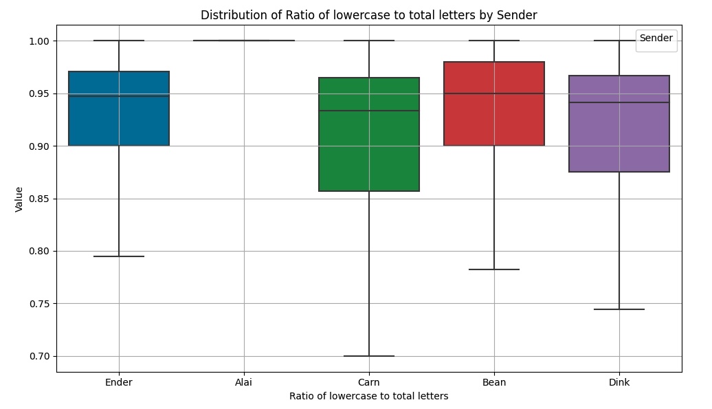
This chart is called a box plot. It shows the distribution (in percentiles) of the value of a variable. Higher values of this feature mean that a given sender tended to send messages with fewer uppercase letters. Values close to 1 mean that a message almost never used uppercase letters - maybe because it was a long sentence or the sender didn’t bother to capitalize. Values farther from 1 mean that a message contains a lot of caps - maybe the sender was ANGRY or wrote in short sentences. From looking at the plot you can see that Alai has a very different capitalization pattern than the rest of the senders. We confirm this with the Kruskal-Wallis H test, though this test also has a tendency to give every feature high significance with large data sizes. We use eta-squared to identify the magnitude of the impact this feature has on the sender. P-value is again 0.00000 and the eta-squared for this feature is 0.32. The next highest continuous feature in the dataset has an eta-squared of 0.02!
You can check out the Feature Extraction Notebook on Github to see how meaningful the rest of my features were. We’ll keep adding to these features as we move through the series, but hopefully this gives you a good idea of what to look for in your own exploration.
Conclusion
In this blog, we discussed what a feature was and how to extract them from your dataset. We noted some important considerations like having a hypothesis for each feature instead of extracting them willy nilly and wrote some code to extract features from our Messages. We talked about the different types of features (numerical and categorical), the specific sources we can use in our dataset (the current message or previous messages), and some categories of features we may consider. We also went through the exercise of extracting and examining a few features that turned out to be meaningful in our dataset. Model building is an iterative process, and as we learn more about our data through the modeling process we’ll add more features to our extraction code.
Now that we have our features extracted, we’re ready to move to our first real model! Next time, we’ll use some basic linear models (y=mx+b stuff) to see how much improvement we can make with traditional methods. Stay tuned for the next post!